mathjax

Showing posts with label graph. Show all posts

Tuesday, May 3, 2011

Structural Similarity With Apache Pig

A while ago I posted this about computing the jaccard similarity (otherwise known as the structural similarity) of nodes in a network graph. Looking back on it over the past few days I realize there are some areas for serious improvement. Actually, it's just completely wrong. The approach is broken. So, I'm going to revisit the algorithm again, in more detail, and write a vastly improved Pig script for computing the structural similarity of vertices in a network graph.

The graph


Of course, before you can do a whole lot of anything, you've got to have a graph to work with. To keep things dead simple (and breaking from what I normally do) I'm going to draw an arbitrary graph (and by draw I mean draw). Here it is:

This can be represented as a tab-separated-values set of adjacency pairs in a file called 'graph.tsv':

$: cat graph.tsv
A C
B C
C D
C E
E F
C H
G H
C G
D E
A G
B G


I don't think it gets any simpler.

The Measure


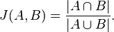
Now, the idea here is to compute the similarity between nodes, eg similarity(A,B). There's already a well defined measure for this called the jaccard similarity. The key take away is to notice that:


The Pig


This can be broken into a set of Pig operations quite easily actually:

load data


Remember, I saved the data into a file called 'graph.tsv'. So:


edges = LOAD 'graph.tsv' AS (v1:chararray, v2:chararray);
edges_dup = LOAD 'graph.tsv' AS (v1:chararray, v2:chararray);


It is necessary, but still a hack, to load the data twice at the moment. This is because self-intersections (which I'll be doing in a moment) don't work with Pig 0.8 at the moment.

augment with sizes


Now I need the 'size' of each of the sets. In this case the 'sets' are the list of nodes each node links to. So, all I really have to do is calculate the number of outgoing links:


grouped_edges = GROUP edges BY v1;
aug_edges = FOREACH grouped_edges GENERATE FLATTEN(edges) AS (v1, v2), COUNT(edges) AS v1_out;

grouped_dups = GROUP edges_dup BY v1;
aug_dups = FOREACH grouped_dups GENERATE FLATTEN(edges_dup) AS (v1, v2), COUNT(edges_dup) AS v1_out;


Again, if self-intersections worked, the operation of counting the outgoing links would only have to happen once. Now I've got a handle on the |A| and |B| parts of the equation above.

intersection


Next I'm going to compute the intersection using a Pig join:


edges_joined = JOIN aug_edges BY v2, aug_dups BY v2;
intersection = FOREACH edges_joined {
--
-- results in:
-- (X, Y, |X| + |Y|)
--
added_size = aug_edges::v1_out + aug_dups::v1_out;
GENERATE
aug_edges::v1 AS v1,
aug_dups::v1 AS v2,
added_size AS added_size
;
};


Notice I'm adding the individual set sizes. This is to come up the |A| + |B| portion of the denominator in the jaccard index.

intersection sizes


In order to compute the size of the intersection I've got to use a Pig GROUP and collect all the elements that matched on the JOIN:


intersect_grp = GROUP intersection BY (v1, v2);
intersect_sizes = FOREACH intersect_grp {
--
-- results in:
-- (X, Y, |X /\ Y|, |X| + |Y|)
--
intersection_size = (double)COUNT(intersection);
GENERATE
FLATTEN(group) AS (v1, v2),
intersection_size AS intersection_size,
MAX(intersection.added_size) AS added_size -- hack, we only need this one time
;
};


There's a hack in there. The reason is that 'intersection.added_size' is a Pig data bag containing some number of identical tuples (equal to the intersection size). Each of these tuples is the 'added_size' from the previous step. Using MAX is just a convenient way of pulling out only one of them.

similarity


And finally, I have all the pieces in place to compute the similarities:


similarities = FOREACH intersect_sizes {
--
-- results in:
-- (X, Y, |X /\ Y|/|X U Y|)
--
similarity = (double)intersection_size/((double)added_size-(double)intersection_size);
GENERATE
v1 AS v1,
v2 AS v2,
similarity AS similarity
;
};


That'll do it. Here's the full script for completeness:


edges = LOAD '$GRAPH' AS (v1:chararray, v2:chararray);
edges_dup = LOAD '$GRAPH' AS (v1:chararray, v2:chararray);

--
-- Augment the edges with the sizes of their outgoing adjacency lists. Note that
-- if a self join was possible we would only have to do this once.
--
grouped_edges = GROUP edges BY v1;
aug_edges = FOREACH grouped_edges GENERATE FLATTEN(edges) AS (v1, v2), COUNT(edges) AS v1_out;

grouped_dups = GROUP edges_dup BY v1;
aug_dups = FOREACH grouped_dups GENERATE FLATTEN(edges_dup) AS (v1, v2), COUNT(edges_dup) AS v1_out;

--
-- Compute the sizes of the intersections of outgoing adjacency lists
--
edges_joined = JOIN aug_edges BY v2, aug_dups BY v2;
intersection = FOREACH edges_joined {
--
-- results in:
-- (X, Y, |X| + |Y|)
--
added_size = aug_edges::v1_out + aug_dups::v1_out;
GENERATE
aug_edges::v1 AS v1,
aug_dups::v1 AS v2,
added_size AS added_size
;
};

intersect_grp = GROUP intersection BY (v1, v2);
intersect_sizes = FOREACH intersect_grp {
--
-- results in:
-- (X, Y, |X /\ Y|, |X| + |Y|)
--
intersection_size = (double)COUNT(intersection);
GENERATE
FLATTEN(group) AS (v1, v2),
intersection_size AS intersection_size,
MAX(intersection.added_size) AS added_size -- hack, we only need this one time
;
};

similarities = FOREACH intersect_sizes {
--
-- results in:
-- (X, Y, |X /\ Y|/|X U Y|)
--
similarity = (double)intersection_size/((double)added_size-(double)intersection_size);
GENERATE
v1 AS v1,
v2 AS v2,
similarity AS similarity
;
};

DUMP similarities;


Results


Run it:


$: pig -x local jaccard.pig
...snip...
(A,A,1.0)
(A,B,1.0)
(A,C,0.2)
(B,A,1.0)
(B,B,1.0)
(B,C,0.2)
(C,A,0.2)
(C,B,0.2)
(C,C,1.0)
(C,D,0.25)
(C,G,0.25)
(D,C,0.25)
(D,D,1.0)
(E,E,1.0)
(G,C,0.25)
(G,G,1.0)


And it's done! Hurray. Now, go make a recommender system or something.

Friday, February 4, 2011

Brute Force Graph Crunching With Pig and Wukong

Just discovered this amazing data set matching all Marvel Universe comic book characters with the comic books they've appeared in (Social Characteristics of the Marvel Universe). I've made the data set available on Infochimps here in a sane and easy to use format.

Here's what that looks like:

$: head labeled_edges.tsv | wu-lign
"FROST, CARMILLA" "AA2 35"
"KILLRAVEN/JONATHAN R" "AA2 35"
"M'SHULLA" "AA2 35"
"24-HOUR MAN/EMMANUEL" "AA2 35"
"OLD SKULL" "AA2 35"
"G'RATH" "AA2 35"
"3-D MAN/CHARLES CHAN" "M/PRM 35"
"3-D MAN/CHARLES CHAN" "M/PRM 36"
"3-D MAN/CHARLES CHAN" "M/PRM 37"
"HUMAN ROBOT" "WI? 9"


Simple Question


A natural question to ask of such an awesome graph is for the similarity between two characters based on what comic books they've appeared in together. This is called the structural similarity since we're only using the structure of the graph and no other meta data (weights, etc). Note that this could also be applied the other direction to find the similarity between two comic books based on what characters they share.

Wee bit of math


The structural similarity is nothing more than the jaccard similarity applied to nodes in a network graph. Here's the definition of that from wikipedia:


So basically all we've got to do is get a list of all the comic books that two characters, say character A and character B, have appeared in. These lists of comic books form two mathematical sets.

The numerator in that simple formula says to compute the intersection of A and B and then count how many elements are left. More plainly, that's just the number of comic books the two characters have in common.

The denominator tells us to compute the union of A and B and count how many elements are in the resulting set. That's just the number of unique comic books that A and B have ever been in, either at the same time or not.

Pig


Here how we're going to say it using pig:


DEFINE jaccard_similarity `ruby jaccard_similarity.rb --map` SHIP('jaccard_similarity.rb');
edges = LOAD '/data/comics/marvel/labeled_edges.tsv' AS (character:chararray, comic:chararray);
grouped = GROUP edges BY character;
with_sets = FOREACH grouped GENERATE group AS character, FLATTEN(edges.comic) AS comic, edges.comic AS set;
SPLIT with_sets INTO with_sets_dup IF ( 1 > 0 ), not_used if (1 < 0); -- hack hack hack, self join still doesn't work
joined = JOIN with_sets BY comic, with_sets_dup BY comic;
pairs = FOREACH joined GENERATE
with_sets::character AS character_a,
with_sets::set AS character_a_set,
with_sets_dup::character AS character_b,
with_sets_dup::set AS character_b_set
;
similarity = STREAM pairs THROUGH jaccard_similarity AS (character_a:chararray, character_b:chararray, similarity:float);
STORE similarity INTO '/data/comics/marvel/character_similarity.tsv';


Notice we're doing a bit of funny business here. Writing the actual algorithm for the jaccard similarity between two small sets doesn't make much sense in Pig. Instead we've written a wukong script to do it for us (you could also write a Pig udf if you're a masochist).

The first thing we do here is use the DEFINE operator to tell pig that there's an external command we want to call, the alias for it, how to call it, and to SHIP the script we need to all nodes in the cluster.

Next we use the GROUP operator and then the FOREACH..GENERATE projection operator to get, for every character, a the list of comic books they've appeared in.

We also use the FLATTEN operator during the projection as well. The reason is so that we can use the JOIN operator to pull out (character,character) pairs that have at least one comic book in common. (Don't get scared about the gross looking SPLIT operator in there. Just ignore it. It's a hack to get around the fact that self-joins still don't quite work properly in pig. Pretend we're just joining 'with_sets' with itself.)

The last step is to STREAM our pairs through the simple wukong script. Here's what that looks like:


#!/usr/bin/env ruby

require 'rubygems'
require 'wukong'
require 'wukong/and_pig' # for special conversion methods
require 'set'

#
# Takes two pig bags and computes their jaccard similarity
#
# eg.
#
# input:
#
# (a,{(1),(2),(3)}, b, {(2),(9),(5)})
#
# output:
#
# (a, b, 0.2)
#
class JaccardSim < Wukong::Streamer::RecordStreamer
def process node_a, set_a, node_b, set_b
yield [node_a, node_b, jaccard(set_a, set_b)]
end

def jaccard bag_a, bag_b
common_elements = ((bag_a.from_pig_bag.to_set).intersection(bag_b.from_pig_bag.to_set)).size
total_elements = ((bag_a.from_pig_bag.to_set).union(bag_b.from_pig_bag.to_set)).size
common_elements.to_f / total_elements.to_f
end
end

Wukong::Script.new(JaccardSim, nil).run


Notice the nifty 'from_pig_bag' method that wukong has. All we're doing here is converting the two pig bags into ruby 'set' objects then doing the simple jaccard similarity calculation. (3 lines of code for the calculation itself, still want to do it in java?)

And that's it. Here's what it looks like after running:


"HUMAN TORCH/JOHNNY S" "GALACTUS/GALAN" 0.0514112900
"HUMAN TORCH/JOHNNY S" "ROGUE /" 0.0371308030
"HUMAN TORCH/JOHNNY S" "UATU" 0.0481557360
"LIVING LIGHTNING/MIG" "USAGENT DOPPELGANGER" 0.0322580640
"LIVING LIGHTNING/MIG" "STRONG GUY/GUIDO CAR" 0.1052631600
"LIVING LIGHTNING/MIG" "STORM/ORORO MUNROE S" 0.0209059230
"LIVING LIGHTNING/MIG" "USAGENT/CAPTAIN JOHN" 0.1941747500
"LIVING LIGHTNING/MIG" "WASP/JANET VAN DYNE " 0.0398089180
"LIVING LIGHTNING/MIG" "THING/BENJAMIN J. GR" 0.0125120310
"LIVING LIGHTNING/MIG" "WOLFSBANE/RAHNE SINC" 0.0209059230
"LIVING LIGHTNING/MIG" "THUNDERSTRIKE/ERIC K" 0.1153846160
"LIVING LIGHTNING/MIG" "WILD CHILD/KYLE GIBN" 0.0434782600


Sweet.

Thursday, January 20, 2011

Graph Processing With Wukong and Hadoop

As a last (for now) tutorial oriented post on Wukong, let's process a network graph.

Get Data


This airport data (airport edges) from Infochimps is one such network graph with over 35 million edges. It represents the number of flights and passengers transported between two domestic airports in a given month. Go ahead and download it.

Explore Data


We've got to actually look at the data before we can make any decisions about how to process it and what questions we'd like answered:


$: head data/flights_with_colnames.tsv | wu-lign
origin_airport destin_airport passengers flights month
MHK AMW 21 1 200810
EUG RDM 41 22 199011
EUG RDM 88 19 199012
EUG RDM 11 4 199010
MFR RDM 0 1 199002
MFR RDM 11 1 199003
MFR RDM 2 4 199001
MFR RDM 7 1 199009
MFR RDM 7 2 199011


So it's exactly what you'd expect; An adjacency list with (origin node,destination node,weight_1,weight_2,timestamp). There are thousands of data sets with similar characteristics...

Ask A Question


A simple question to ask (and probably the first question you should ask of a graph) is what the degree distribution is. Notice there are two flavors of degree in our graph:

1. Passenger Degree: For a given airport (node in the graph) the number of passengers in + the number of passengers out. Passengers in is called the 'in degree' and passengers out is (naturally) called the 'out degree'.

2. Flights Degree: For a given airport the number of flights in + the number of flights out.

Let's write the question wukong style:

#!/usr/bin/env ruby

require 'rubygems'
require 'wukong'

class EdgeMapper < Wukong::Streamer::RecordStreamer
#
# Yield both ways so we can sum (passengers in + passengers out) and (flights
# in + flights out) individually in the reduce phase.
#
def process origin_code, destin_code, passengers, flights, month
yield [origin_code, month, "OUT", passengers, flights]
yield [destin_code, month, "IN", passengers, flights]
end
end

class DegreeCalculator < Wukong::Streamer::AccumulatingReducer
#
# What are we going to use as a key internally?
#
def get_key airport, month, in_or_out, passengers, flights
[airport, month]
end

def start! airport, month, in_or_out, passengers, flights
@out_degree = {:passengers => 0, :flights => 0}
@in_degree = {:passengers => 0, :flights => 0}
end

def accumulate airport, month, in_or_out, passengers, flights
case in_or_out
when "IN" then
@in_degree[:passengers] += passengers.to_i
@in_degree[:flights] += flights.to_i
when "OUT" then
@out_degree[:passengers] += passengers.to_i
@out_degree[:flights] += flights.to_i
end
end

#
# For every airport and month, calculate passenger and flight degrees
#
def finalize

# Passenger degrees (out, in, and total)
passengers_out = @out_degree[:passengers]
passengers_in = @in_degree[:passengers]
passengers_total = passengers_in + passengers_out

# Flight degrees (out, in, and total)
flights_out = @out_degree[:flights]
flights_in = @in_degree[:flights]
flights_total = flights_in + flights_out

yield [key, passengers_in, passengers_out, passengers_total, flights_in, flights_out, flights_total]
end
end

#
# Need to use 2 fields for partition so every record with the same airport and
# month land on the same reducer
#
Wukong::Script.new(
EdgeMapper,
DegreeCalculator,
:partition_fields => 2 # use two fields to partition records
).run


Don't panic. There's a lot going on in this script so here's the breakdown (real gentle like):

Mapper


Here we're using wukong's RecordStreamer class which reads lines from $stdin and splits on tabs for us already. That's how we know exactly what arguments the process method gets.

Next, as is often the case with low level map-reduce, we've got to be a bit clever in the way we yield data in the map. Here we yield the edge both ways and attach an extra piece of information ("OUT" or "IN") depending on whether the passengers and flights were going into the airport in a month or out. This way we can distinguish between these two pieces of data in the reducer and process them independently.

Finally, we've carefully rearranged our records such that (airport,month) is always the first two fields. We'll partition on this as the key. (We have to say that explicitly at the bottom of the script)

Reducer


We've seen all these methods before except for one. The reducer needs to know what fields to use as the key (it defaults to the first field). Here we've explicitly told it to use the airport and month as the key with the 'get_key' method.

* start! - Here we initialize the internal state of the reducer with two ruby hashes. One, the @out_degree will count up all the passengers and flights out. The @in_degree will do the same but for passengers and flights in. (Let's all take a moment and think about how awful and unreadable that would be in java...)

* accumulate - Here we simply look at each record and decide which counters to increment depending on whether it's "OUT" or "IN".

* finalize - All we're doing here is taking our accumulated counts, creating the record we care about, and yielding it out. Remember, the 'key' is just (airport,month).

Get An Answer


We know how to put the data on the hdfs and run the script by now so we'll skip that part. Here's what the output looks like:


$: hdp-catd /data/domestic/flights/degree_distribution | head -n20 | wu-lign
1B1 200906 1 1 2 1 1 2
ABE 200705 0 83 83 0 3 3
ABE 199206 0 31 31 0 1 1
ABE 200708 0 904 904 0 20 20
ABE 200307 0 91 91 0 2 2
ABE 200703 0 36 36 0 1 1
ABE 199902 0 84 84 0 1 1
ABE 200611 0 753 753 0 18 18
ABE 199209 0 99 99 0 1 1
ABE 200702 0 54 54 0 1 1
ABE 200407 0 98 98 0 1 1
ABE 200705 0 647 647 0 15 15
ABE 200306 0 27 27 0 1 1
ABE 200703 0 473 473 0 11 11
ABE 200309 0 150 150 0 1 1
ABE 200702 0 313 313 0 8 8
ABE 200103 0 0 0 0 1 1
ABE 199807 0 105 105 0 1 1
ABE 199907 0 91 91 0 1 1
ABE 199501 0 50 50 0 1 1


At this point is where you might bring this back down to your local file system, crack open a program like R, make some plots, etc.

And we're done for now. Hurray.

Thursday, January 13, 2011

Plot a FIFO in R

Recently discovered a really simple way to plot a fifo in rstats. Here's a simple example of plotting the output of your ifstat program. From one terminal do:


mkfifo ifstat_fifo
ifstat -n > ifstat_fifo


Then, in another terminal, open an R shell and do the following:


# Plot the most recent 100 seconds of inbound network traffic
> while(T){
d <- read.table(fifo("ifstat_fifo",open="read"))
x <- rbind(x,d)
x <-tail(x,100)
plot(x$V1,type='l')
Sys.sleep(1)
}


You may have to run it a couple times while the fifo fills with data. And here's what that looks like: